Natural Graph Networks: A Fresh Take on Graph Neural Networks
Written by: Claude Sonnet 4
Directed by:
- Chaohui Guo
- TC Chen
- Daniel Daza
Graph Neural Networks (GNNs) have become a cornerstone of machine learning on graphs, but they suffer from fundamental limitations that restrict their expressiveness. A 2020 NeurIPS paper by Pim de Haan, Taco Cohen, and Max Welling introduces Natural Graph Networks (NGNs), a novel approach that addresses these limitations by thinking about graph learning in terms of local message passing on edge neighborhoods rather than traditional node-centric approaches.
The Problem with Traditional GNNs
To understand why NGNs matter, let’s first examine what’s wrong with standard Graph Neural Networks like GCNs (Graph Convolutional Networks) and GraphSAGE.
Traditional GNNs follow a simple recipe:
- Each node aggregates features from its neighbors
- The aggregated features are transformed through a neural network
- This process repeats for multiple layers
Mathematically, a standard GNN layer can be written as:
\[h_i^{(l+1)} = \sigma\left(W^{(l)} \cdot \text{AGG}\left(\{h_j^{(l)} : j \in \mathcal{N}(i)\}\right)\right)\]where $h_i^{(l)}$ is the feature vector of node $i$ at layer $l$, $\mathcal{N}(i)$ are the neighbors of node $i$, and AGG is some aggregation function like mean or sum.
The fundamental problem: This approach has limited expressive power. The seminal work by Xu et al. (2019) proved that standard GNNs cannot distinguish between certain graph structures that are fundamentally different. In particular, they’re limited by the 1-Weisfeiler-Lehman (1-WL) test - they can only distinguish graphs that the 1-WL algorithm can distinguish.
Enter Natural Graph Networks: A Local Perspective
Natural Graph Networks take a radically different approach. Instead of thinking about message passing between individual nodes, NGNs focus on edge neighborhoods and use local subgraph processing.
The Core Idea: Edge-Centric Message Passing
The key insight is this: for every directed edge $p \to q$ in a graph, NGNs:
- Extract a local neighborhood: Collect all nodes within $k$ hops of either $p$ or $q$
- Create markers: Add special “marker” features that identify which nodes are $p$ and $q$ in this subgraph
- Process locally: Run a message network (typically a small GNN) on this marked subgraph
- Extract the message: Take the output features at node $q$ as the message $m_{p \to q}$
- Aggregate: Sum all incoming messages at each node
Mathematically, the message from node $p$ to node $q$ is:
\[m_{p \to q} = \text{MessageNet}\left(\mathcal{G}_{pq}^{(k)}, \mathbf{X}_{pq} \oplus \mathbf{M}_{pq}\right)[q]\]where:
- $\mathcal{G}_{pq}^{(k)}$ is the $k$-hop neighborhood around edge $(p,q)$
- $\mathbf{X}_{pq}$ are the node features in this subgraph
- $\mathbf{M}_{pq}$ are binary marker features indicating nodes $p$ and $q$
- $[q]$ extracts the features at position $q$ in the subgraph
Why This Works: Higher-Order Structure Awareness
The magic of this approach lies in its ability to capture higher-order graph structure. While traditional GNNs only see immediate neighbors at each step, NGNs see the entire $k$-hop neighborhood structure around each edge in a single operation.
Consider two graphs where traditional GNNs would produce identical node embeddings but NGNs would not:
Graph A:     Graph B:
  1---2        1---2
  |   |        |\ /|
  3---4        | X |
               |/ \|
               3---4
A traditional GNN sees the same local structure around each node in both graphs. But an NGN processing edge $1 \to 2$ sees different 2-hop neighborhoods: in Graph A, there are two 4-paths from 1 to 2, while in Graph B, there’s a direct 2-path plus longer paths through the crossing pattern.
Implementation: How It Works in Practice
Let’s look at how this is implemented in practice, based on the code in the repository.
Edge Neighborhood Construction
The first step is building the $k$-hop edge neighborhood. For an edge $p \to q$, this means finding all nodes that are within $k$ steps of either $p$ or $q$:
def edge_neighborhood_nodes(G, p, q, k=1):
    """Find all nodes within k hops of p or q"""
    def within_k(start):
        visited = {start}
        frontier = {start}
        for _ in range(k):
            next_nodes = set()
            for u in frontier:
                next_nodes.update(G.neighbors(u))
            next_nodes -= visited
            visited |= next_nodes
            frontier = next_nodes
        return visited

    return within_k(p) | within_k(q)  # Union of both neighborhoods
Marker Features: Telling the Network What to Focus On
The crucial innovation is the marker features. After extracting the edge neighborhood subgraph, NGNs append two binary channels to the node features:
- Channel 1: Set to 1 for node $p$, 0 elsewhere
- Channel 2: Set to 1 for node $q$, 0 elsewhere
def add_marker_features(X, p_sub, q_sub):
    """Add binary marker channels for p and q"""
    m, d = X.shape
    markers = np.zeros((m, 2))
    markers[p_sub, 0] = 1.0  # Mark p
    markers[q_sub, 1] = 1.0  # Mark q
    return np.concatenate([X, markers], axis=1)
These markers are critical - they tell the message network “pay attention to the relationship between these two specific nodes” in the context of their neighborhood structure.
The Message Network
The message network itself can be any graph neural network. In the paper’s implementation, it’s a simple 2-layer GCN:
class MessageGCN(nn.Module):
    def __init__(self, in_dim, hidden_dim, out_dim):
        super().__init__()
        self.gcn1 = GCNLayer(in_dim, hidden_dim)    # in_dim includes +2 for markers
        self.gcn2 = GCNLayer(hidden_dim, out_dim)

    def forward(self, x, adj):
        h = F.relu(self.gcn1(x, adj))
        return self.gcn2(h, adj)
Putting It All Together
The complete NGN layer processes each directed edge in the graph:
def forward(self, G, X):
    n, d = X.shape
    output = torch.zeros((n, self.output_dim))

    for p, q in G.edges():
        # Build p->q neighborhood
        subgraph, p_sub, q_sub = build_subgraph_for_edge(G, p, q, k=self.k)
        X_sub = add_marker_features(X[subgraph], p_sub, q_sub)
        A_sub = adjacency_matrix(subgraph)

        # Run message network
        H_sub = self.message_network(X_sub, A_sub)

        # Extract message at q's position and add to q's features
        message_pq = H_sub[q_sub]
        output[q] += message_pq

        # Process reverse direction q->p
        # ... (similar process)

    return output
Theoretical Foundations: Why NGNs Are More Powerful
The power of NGNs comes from their ability to capture local graph structure in a way that traditional GNNs cannot.
Connection to Higher-Order Graph Properties
Traditional GNNs are fundamentally limited by their locality. At each layer, they can only aggregate information from immediate neighbors. Even with multiple layers, the information flow follows a very specific pattern that misses important structural relationships.
NGNs, on the other hand, look at the complete local structure around each edge. This allows them to detect:
- Triangular patterns: Is edge $(p,q)$ part of triangles? How many?
- Path diversity: Are there multiple paths between $p$ and $q$ through their neighborhood?
- Structural roles: What role do $p$ and $q$ play in their local neighborhood?
Permutation Invariance and Natural Transformations
The “natural” in Natural Graph Networks refers to their connection to category theory and natural transformations. However, you don’t need to understand category theory to appreciate the core insight: NGNs respect the symmetries inherent in graph data.
More concretely, NGNs are permutation invariant - if you relabel the nodes in a graph, the NGN’s output changes in a predictable way that respects the relabeling. This is a stronger guarantee than what standard GNNs provide.
Experimental Results: Do They Actually Work?
The paper demonstrates NGNs’ effectiveness on several benchmarks:
Graph Classification on TU Datasets
The implementation in this repository tests NGNs on 8 standard graph classification datasets from the TU collection:
- MUTAG: Chemical compounds, mutagenic activity prediction
- PROTEINS: Protein structures, enzyme classification
- NCI1/NCI109: Chemical compounds, cancer activity
- IMDB-BINARY/MULTI: Movie collaboration networks
Key Results: NGNs consistently outperform standard GNNs, with particularly strong improvements on datasets where structural properties matter most.
Computational Complexity Trade-offs
The main drawback of NGNs is computational cost. For each edge $(p,q)$, they must:
- Extract a $k$-hop neighborhood (can be expensive for large $k$)
- Run a message network on this subgraph
- Repeat for all edges (potentially O(E) subgraph computations)
In practice, this means NGNs are:
- More expensive than traditional GNNs
- More powerful at capturing structural patterns
- Better suited for smaller graphs where structure matters more than scale
When to Use NGNs
Based on the theoretical insights and experimental results, NGNs are particularly valuable when:
- Structure matters: Your task requires understanding complex topological relationships
- Graphs are reasonably small: The computational overhead is manageable
- Standard GNNs fail: You’ve hit the expressiveness limitations of traditional approaches
- Local patterns are important: Your problem involves detecting specific motifs or structural roles
Implementation Tips and Practical Considerations
If you’re thinking about using NGNs in your own work, here are some practical insights from the codebase:
Neighborhood Size Selection
The choice of $k$ (neighborhood size) is crucial:
- k=1: Captures immediate neighborhood structure, computationally efficient
- k=2: Includes triangles and 4-cycles, good balance of power and efficiency
- k≥3: Very expensive, may suffer from over-smoothing
The paper uses $k=1$ for most experiments, suggesting this is often sufficient.
Message Network Design
The message network doesn’t need to be complex. A simple 2-layer GCN works well:
- Layer 1: Process marked features with neighborhood structure
- Layer 2: Compute final message representation
More complex message networks don’t necessarily help and add computational cost.
Training Considerations
NGNs require some special handling during training:
- Memory usage: Each edge processes its own subgraph, increasing memory requirements
- Batch processing: Hard to batch efficiently due to variable subgraph sizes
- Gradient flow: Messages aggregate additively, which can cause gradient scaling issues
Conclusion: A New Tool for Graph Learning
Natural Graph Networks represent a significant conceptual advance in graph neural networks. By shifting focus from node-centric to edge-centric processing, they unlock new levels of expressiveness that can capture structural patterns invisible to traditional GNNs.
Key Takeaways:
- Higher expressiveness: NGNs can distinguish graph structures that confuse traditional GNNs
- Local structure awareness: They see complete $k$-hop neighborhoods around edges
- Principled design: Based on solid theoretical foundations (natural transformations)
- Practical trade-offs: More powerful but more expensive than standard GNNs
When to consider NGNs:
- Your graphs have rich structural patterns that matter for your task
- Standard GNNs aren’t capturing the relationships you need
- You can afford the computational overhead for better expressiveness
- You’re working with molecular graphs, social networks, or other structure-rich domains
As graph learning continues to evolve, NGNs offer a valuable perspective: sometimes the best way to understand a graph isn’t to think about individual nodes, but to focus on the local structural relationships that give the graph its meaning. In many real-world applications, it’s these local patterns - not global connectivity - that carry the most important information.
The code in this repository provides a clean, educational implementation that makes it easy to experiment with these ideas. Whether you’re a researcher pushing the boundaries of graph learning or a practitioner looking for better tools, Natural Graph Networks deserve a place in your toolkit.


